Incremental Matrix Profiles for Streaming Time Series Data

Now that you have a basic understanding of how to compute a matrix profile, in this short tutorial, we will demonstrate how to incrementally update your matrix profile when you have streaming (on-line) data using the stumpy.stumpi (“STUMP Incremental”) function. You can learn more about the details of this approach by reading Section G of the Matrix Profile I paper and Section 4.6 and Table 5 this paper.

Getting Started

Let’s import the packages that we’ll need to create and analyze a randomly generated time series data set.

import numpy as np
import stumpy
import numpy.testing as npt
import time

Generating Some Random Time Series Data

Imagine that we have an IoT sensor that has been collecting data once an hour for the last 14 days. That would mean that we’ve amassed 14 * 24 = 336 data points up until this point and our data set might look like this:

T = np.random.rand(336)

And, perhaps, we know from experience that an interesting motif or anomaly might be detectable within a 12 hour (sliding) time window:

m = 12

Typical Batch Analysis

To compute the matrix profile using a batch process is straightforward using stumpy.stump:

mp = stumpy.stump(T, m)

But as the length of T grows with each passing hour, it will take increasingly more time to compute the matrix profile since stumpy.stump will actually re-compute all of the pairwise distances between all subsequences within the time series. This is super time consuming! Instead, for streaming data, we want to find a way to take the new incoming (single) data point and compare the subsequence that it resides in with the rest of the time series (i.e., compute the distance profile) and update the existing matrix profile. Luckily, this can be easily accomplished with stumpy.stumpi or “STUMP Incremental”.

Streaming (On-line) Analysis with STUMPI

As we wait for the next data point, t, to arrive, we can take our existing data initialize our streaming object:

stream = stumpy.stumpi(T, m, egress=False)  # Don't egress/remove the oldest data point when streaming

And when a new data point, t, arrives:

t = np.random.rand()

We can append t to our stream and easily update the matrix profile, P, and matrix profile indices, I behind the scenes:

stream.update(t)

In the background, t has been appended to the existing time series and it automatically compares the new subsequence with all of the existing ones and updates the historical values. It also determines which one of the existing subsequences is the nearest neighbor to the new subsequence and appends this information to the matrix profile. And this can continue on, say, for another 1,000 iterations (or indefinitely) as additional data is streamed in:

for i in range(1000):
    t = np.random.rand()
    stream.update(t)

It is important to reiterate that incremental stumpy.stumpi is different from batch stumpy.stump in that it does not waste any time re-computing any of the past pairwise distances. stumpy.stumpi only spends time computing new distances and then updates the appropriate arrays where necessary and, thus, it is really fast!

Validation

The Matrix Profile

Now, this claim of “fast updating” with streaming (on-line) data may feel strange or seem magical so, first, let’s validate that the output from incremental stumpy.stumpi is the same as performing batch stumpy.stump. Let’s start with the full time series with 64 data points and compute the full matrix profile:

T_full = np.random.rand(64)
m = 8

mp = stumpy.stump(T_full, m)
P_full = mp[:, 0]
I_full = mp[:, 1]

Next, for stumpy.stumpi, we’ll only start with the first 10 elements from the full length time series and then incrementally stream in the additional data points one at a time:

# Start with half of the full length time series and initialize inputs
T_stream = T_full[:10].copy()
stream = stumpy.stumpi(T_stream, m, egress=False)  # Don't remove/egress the oldest data point when streaming

# Incrementally add one new data point at a time and update the matrix profile
for i in range(len(T_stream), len(T_full)):
    t = T_full[i]
    stream.update(t)

Now that we’re done, let’s check and validate that:

1. stream.T == T_full

2. stream.P == P_full

3. stream.I == I_full

npt.assert_almost_equal(stream.T_, T_full)
npt.assert_almost_equal(stream.P_, P_full)
npt.assert_almost_equal(stream.I_, I_full)

There are no errors! So, this means that stump.stumpi indeed produces the correct matrix profile results that we’d expect.

The Performance

We’ve basically claimed that incrementally updating our matrix profile with stumpy.stumpi is much faster (in total computational time) than performing a full pairwise distance calculation with stumpy.stump as each new data point arrives. Let’s actually compare the timings by taking a full time series that is 10,000 data points in length and we initialize both approaches with the first 2% of the time series (i.e., the first 200 points) and append a single new data point at each iteration before re-computing the matrix profile:

T_full = np.random.rand(10_000)
T_stream = T_full[:200].copy()
m = 100

# `stumpy.stump` timing
start = time.time()
mp = stumpy.stump(T_stream, m)
for i in range(200, len(T_full)):
    T_stream = np.append(T_stream, T_full[i])
    mp = stumpy.stump(T_stream, m)
stump_time = time.time() - start

# `stumpy.stumpi` timing
stream = stumpy.stumpi(T_stream, m, egress=False)  # Don't egress/remove the oldest data point when streaming
start = time.time()
for i in range(200, len(T_full)):
    t = T_full[i]
    stream.update(t)
stumpi_time = time.time() - start

print(f"stumpy.stump: {np.round(stump_time,1)}s")
print(f"stumpy.stumpi: {np.round(stumpi_time, 1)}s")

stumpy.stump: 257.4s
stumpy.stumpi: 3.1s

Setting aside the fact that having more CPUs will speed up both approaches, we clearly see that incremental stumpy.stumpi is one to two orders of magnitude faster than batch stumpy.stump for processing streaming data. In fact for the current hardware, on average, it is taking roughly 0.1 seconds for stumpy.stump to analyze each new matrix profile. So, if you have more than 10 new data point arriving every second, then you wouldn’t be able to keep up. In contrast, stumpy.stumpi should be able to comfortably handle and process ~450+ new data points per second using fairly modest hardware. Additionally, batch stumpy.stump, which has a computational complexity of O(n^2), will get even slower as more and more data points get appended to the existing time series while stumpy.stumpi, which is essentially O(1), will continue to be highly performant.

In fact, if you don’t care about maintaining the oldest data point and its relationships with the newest data point (i.e., you only care about maintaining a fixed sized sliding window), then you can get slightly improve the performance by telling stumpy.stumpi to remove/egress the oldest data point (along with its corresponding matrix profile information) by setting the parameter egress=True when we instantiate our streaming object (note that this is actually the default behavior):

stream = stumpy.stumpi(T_stream, m, egress=True)  # Egressing/removing the oldest data point is the default behavior!

And now, when we process the same data above:

# `stumpy.stumpi` timing with egress
stream = stumpy.stumpi(T_stream, m, egress=True)
start = time.time()
for i in range(200, len(T_full)):
    t = T_full[i]
    stream.update(t)
stumpi_time = time.time() - start

print(f"stumpy.stumpi: {np.round(stumpi_time, 1)}s")

stumpy.stumpi: 3.4s

A Visual Example

Now that we understand how to compute and update our matrix profile with streaming data, let’s explore this with a real example data set where there is a known pattern and see if stumpy.stumpi can correctly identify when the global pattern (motif) is encountered.

Retrieving and Loading the Data

First let’s import some additional Python packages and then retrieve our standard “Steamgen Dataset”:

%matplotlib inline

import pandas as pd
import stumpy
import numpy as np
import matplotlib.pyplot as plt
from matplotlib.patches import Rectangle
from matplotlib import animation
from IPython.display import HTML
import os

plt.style.use('https://raw.githubusercontent.com/TDAmeritrade/stumpy/main/docs/stumpy.mplstyle')

steam_df = pd.read_csv("https://zenodo.org/record/4273921/files/STUMPY_Basics_steamgen.csv?download=1")
steam_df.head()

	drum pressure	excess oxygen	water level	steam flow
0	320.08239	2.506774	0.032701	9.302970
1	321.71099	2.545908	0.284799	9.662621
2	320.91331	2.360562	0.203652	10.990955
3	325.00252	0.027054	0.326187	12.430107
4	326.65276	0.285649	0.753776	13.681666

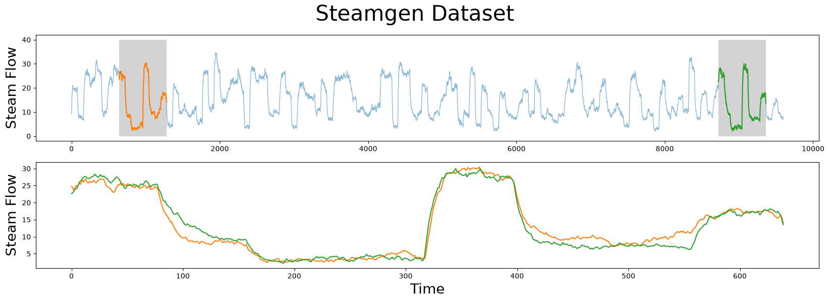
This data was generated using fuzzy models applied to mimic a steam generator at the Abbott Power Plant in Champaign, IL. The data feature that we are interested in is the output steam flow telemetry that has units of kg/s and the data is “sampled” every three seconds with a total of 9,600 datapoints.

The motif (pattern) that we are looking for is highlighted below and yet it is still very hard to be certain that the orange and green subsequences are a match, that is, until we zoom in on them and overlay the subsequences on top each other. Now, we can clearly see that the motif is very similar!

m = 640
fig, axs = plt.subplots(2)
plt.suptitle('Steamgen Dataset', fontsize='30')
axs[0].set_ylabel("Steam Flow", fontsize='20')
axs[0].plot(steam_df['steam flow'], alpha=0.5, linewidth=1)
axs[0].plot(steam_df['steam flow'].iloc[643:643+m])
axs[0].plot(steam_df['steam flow'].iloc[8724:8724+m])
rect = Rectangle((643, 0), m, 40, facecolor='lightgrey')
axs[0].add_patch(rect)
rect = Rectangle((8724, 0), m, 40, facecolor='lightgrey')
axs[0].add_patch(rect)
axs[1].set_xlabel("Time", fontsize='20')
axs[1].set_ylabel("Steam Flow", fontsize='20')
axs[1].plot(steam_df['steam flow'].values[643:643+m], color='C1')
axs[1].plot(steam_df['steam flow'].values[8724:8724+m], color='C2')
plt.show()

Using STUMPI

Now, let’s take a look at what happens to the matrix profile when we initialize our stumpy.stumpi with the first 2,000 data points:

T_full = steam_df['steam flow'].values
T_stream = T_full[:2000]
stream = stumpy.stumpi(T_stream, m, egress=False)  # Don't egress/remove the oldest data point when streaming

and then incrementally append a new data point and update our results:

windows = [(stream.P_, T_stream)]
P_max = -1
for i in range(2000, len(T_full)):
    t = T_full[i]
    stream.update(t)

    if i % 50 == 0:
        windows.append((stream.P_, T_full[:i+1]))
        if stream.P_.max() > P_max:
            P_max = stream.P_.max()

When we plot the growing time series (upper panel), T_stream, along with the matrix profile (lower panel), P, we can watch how the matrix profile evolves as new data is appended:

fig, axs = plt.subplots(2, sharex=True, gridspec_kw={'hspace': 0})

rect = Rectangle((643, 0), m, 40, facecolor='lightgrey')
axs[0].add_patch(rect)
rect = Rectangle((8724, 0), m, 40, facecolor='lightgrey')
axs[0].add_patch(rect)
axs[0].set_xlim((0, T_full.shape[0]))
axs[0].set_ylim((-0.1, T_full.max()+5))
axs[1].set_xlim((0, T_full.shape[0]))
axs[1].set_ylim((-0.1, P_max+5))
axs[0].axvline(x=643, linestyle="dashed")
axs[0].axvline(x=8724, linestyle="dashed")
axs[1].axvline(x=643, linestyle="dashed")
axs[1].axvline(x=8724, linestyle="dashed")
axs[0].set_ylabel("Steam Flow", fontsize='20')
axs[1].set_ylabel("Matrix Profile", fontsize='20')
axs[1].set_xlabel("Time", fontsize='20')


lines = []
for ax in axs:
    line, = ax.plot([], [], lw=2)
    lines.append(line)
line, = axs[1].plot([], [], lw=2)
lines.append(line)

def init():
    for line in lines:
        line.set_data([], [])
    return lines

def animate(window):
    P, T = window
    for line, data in zip(lines, [T, P]):
        line.set_data(np.arange(data.shape[0]), data)

    return lines

anim = animation.FuncAnimation(fig, animate, init_func=init,
                               frames=windows, interval=100,
                               blit=True, repeat=False)

anim_out = anim.to_jshtml()
plt.close()  # Prevents duplicate image from displaying
if os.path.exists("None0000000.png"):
    os.remove("None0000000.png")  # Delete rogue temp file

HTML(anim_out)
# anim.save('/tmp/stumpi.mp4')

Once Loop Reflect

Here, the vertical dotted lines mark the position of where the global motif pair is expected to be and the gray box emphasizes the corresponding motif subsequences. As you play through this animation you may notice that the matrix profile is constantly changing since past subsequences may find a new nearest neighbor. However, note that any change in the matrix profile can only move downward (toward zero). Throughout most of this animation, the subsequence highlighted on the left (grey box) has a relatively high matrix profile value. However, as the time series extends past the grey box on the right, the aforementioned matrix profile value drops significantly and stabilizes quickly as soon as its nearest neighbor has fully arrived in the stream. This is really cool! In fact, the authors of the original Matrix Profile I paper point out that, on this dataset, it would be possible to continue monitoring the matrix profile with stumpy.stumpi for several decades before running out of time or memory!

Bonus Section - Never Update History

Above, we’ve gone with the typical definition of a matrix profile. That is, for any given subsequence, T[i : i + m], find the distance to its nearest neighbor, T[j : j + m], regardless of whether j is to the left of i (i.e., j < i) or to the right of i (i.e., j > i). This means that as new data comes in, even the matrix profiles for the past historical data points also get updated if a “new” nearest neighbor has revealed itself. Essentially, this is “hindsight”. So, there may be a case where, the first time you see a unique subsequence, you may identify it as an anomaly due to its relatively high matrix profile value. However, as more and more new data arrive, this originally anomalous subsequence may no longer be unique anymore. Consider observing only the first period of a sine wave, all of these subsequence would be unique. But as the next period of the sine wave starts to stream in, we realize that the data points in the first period are no longer anomalous so we update their matrix profile values accordingly.

Now, this may or may not be beneficial depending on how you choose to define an “anomaly”. In fact, you may choose not to update the matrix profiles from the past and you may want to restrict the search for a nearest neighbor, j, to always be to the left of i (i.e., j < i). Luckily, in stumpy.stumpi this is already done for you and you can access the left matrix profile and the left matrix profile indices via the .left_P and the .left_I attributes, respectively, of your streaming object:

T_full = np.random.rand(64)
m = 8

T_stream = T_full[:10].copy()
stream = stumpy.stumpi(T_stream, m, egress=False)  # Don't egress/remove the oldest data point when streaming. To egress, set `egress=True`

for i in range(len(T_stream), len(T_full)):
    t = T_full[i]
    stream.update(t)

print(f"Full Matrix Profile: {np.round(stream.P_, 2)}")
print(f"Left Matrix Profile: {np.round(stream.left_P_, 2)}")
print(f"Full Matrix Profile Indices: {stream.I_}")
print(f"Left Matrix Profile Indices: {stream.left_I_}")

Full Matrix Profile: [1.78 1.53 1.49 1.19 2.13 1.66 2.5  2.35 1.94 2.29 2.35 2.33 1.97 1.66
 2.14 2.77 1.99 1.94 2.59 2.53 2.56 2.7  2.27 2.23 2.13 1.4  1.97 1.92
 2.35 1.88 1.81 2.12 2.19 2.3  1.78 1.75 1.39 2.5  2.14 1.94 2.29 2.35
 2.15 1.85 1.95 1.16 1.39 2.21 2.35 1.88 1.81 1.99 2.4  2.15 1.53 1.49
 1.16]
Left Matrix Profile: [ inf  inf  inf 2.81 3.75 4.04 3.53 3.7  3.65 2.92 2.79 2.61 2.39 1.66
 2.72 2.77 3.01 2.96 2.94 2.53 2.62 2.7  2.33 2.71 2.67 1.4  1.97 1.92
 2.56 2.47 2.27 2.23 2.19 2.3  1.78 1.75 2.34 2.5  2.14 1.94 2.29 2.35
 2.55 2.39 2.13 1.8  1.39 2.21 2.35 1.88 1.81 1.99 2.4  2.15 1.53 1.49
 1.16]
Full Matrix Profile Indices: [34 54 55 56 46 13 37 38 39 40 41 22 26  5 38 39 51 55 56  4 28 10 30 31
 44  3 12  5 48 49 50 49 24 25  0  1 46  6 14  8  9 10 53 54 55 56 36 36
 28 29 30 16  7 42  1  2 45]
Left Matrix Profile Indices: [-1 -1 -1  0  1  2  3  4  5  1  2  3  4  5 10 11  9  2  3  4  9 10 11  9
 10  3 12  5 20  7 22 23 24 25  0  1  4  6 14  8  9 10 11 34 24  3 36 36
 28 29 30 16  7 42  1  2 45]

Of course, it is important to point out that a -1 value in the left matrix profile indices does not correspond to the last subsequence in the time series. Instead, it means that the subsequence in that position has no valid nearest neighbor to its left. Consequently, the corresponding left matrix profile value will be set to np.inf.

Summary

And that’s it! You’ve just learned how to incrementally update your matrix profile for streaming (on-line) data.

Resources

Matrix Profile I

Time Series Joins, Motifs, Discords and Shapelets: A Unifying View that Exploits the Matrix Profile (see Section 4.6 and Table 5)

STUMPY Documentation

STUMPY Matrix Profile Github Code Repository