The Matrix Profile#
Laying the Foundation#
At its core, the STUMPY library efficiently computes something called a matrix profile, a vector that stores the z-normalized Euclidean distance between any subsequence within a time series and its nearest neighbor.
To fully understand what this means, let’s take a step back and start with a simple illustrative example along with a few basic definitions:
Time Series with Length n = 13#
time_series = [0, 1, 3, 2, 9, 1, 14, 15, 1, 2, 2, 10, 7]
n = len(time_series)
To analyze this time series with length n = 13, we could visualize the data or calculate global summary statistics (i.e., mean, median, mode, min, max). If you had a much longer time series, then you may even feel compelled to build an ARIMA model, perform anomaly detection, or attempt a forecasting model but these methods can be complicated and may often have false positives or no interpretable insights.

However, if we were to apply Occam’s Razor, then what is the most simple and intuitive approach that we could take analyze to this time series?
To answer this question, let’s start with our first defintion:
Subsequence /ˈsəbsəkwəns/ noun#
a part or section of the full time series#
So, the following are all considered subsequences of our time_series since they can all be found in the time series above.
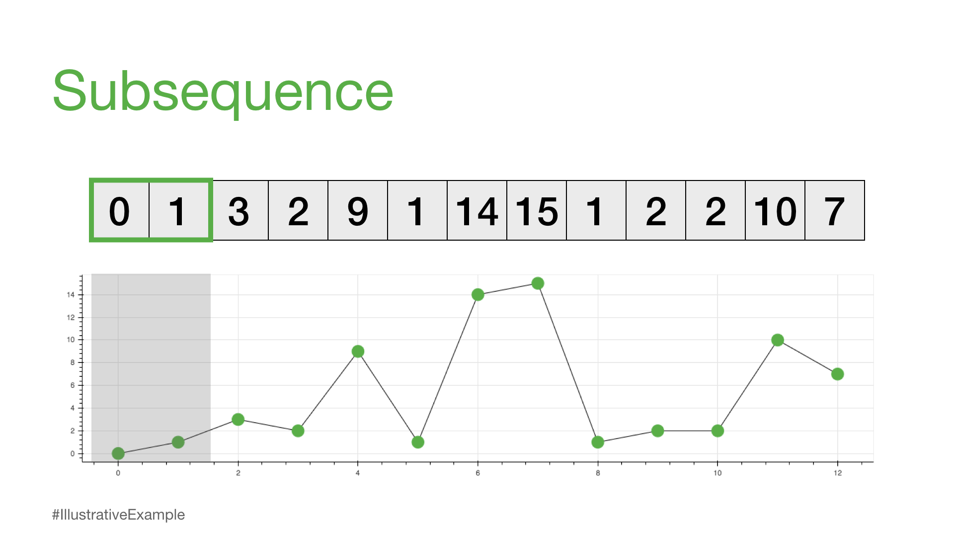
print(time_series[0:2])
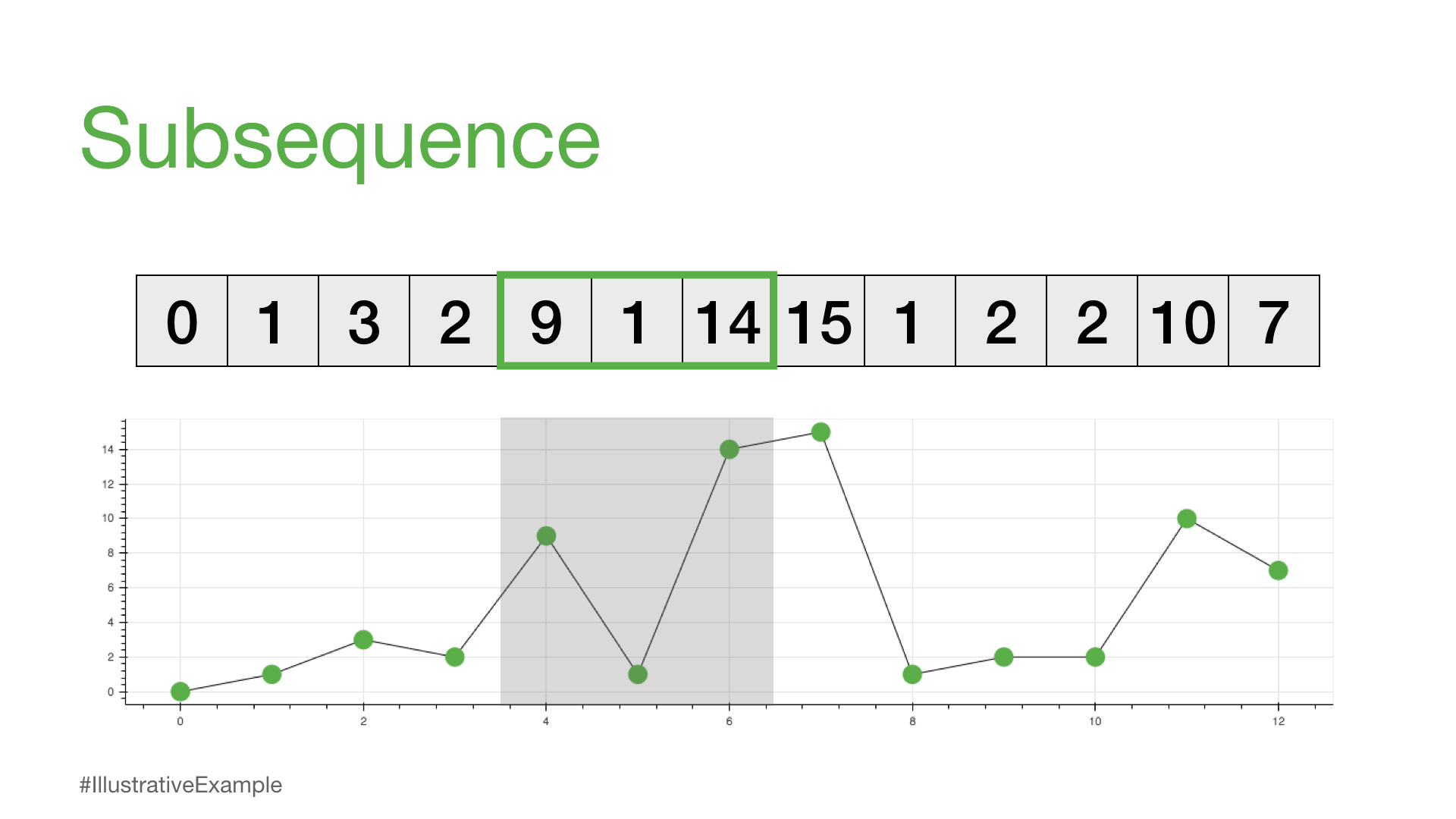
print(time_series[4:7])
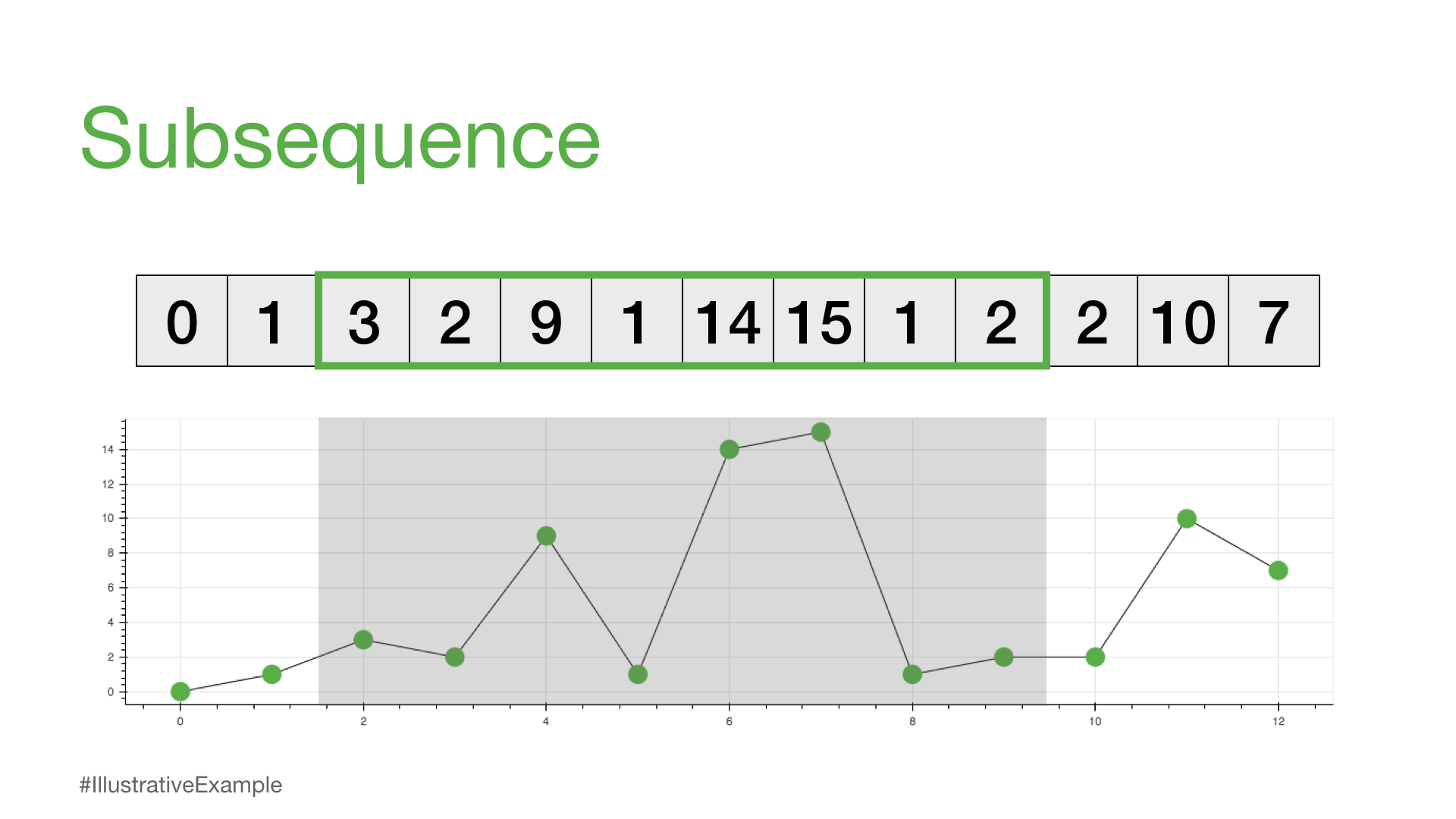
print(time_series[2:10])
[0, 1]
[9, 1, 14]
[3, 2, 9, 1, 14, 15, 1, 2]
We can see that each subsequence can have a different sequence length that we’ll call m. So, for example, if we choose m = 4, then we can think about how we might compare any two subsequences of the same length.
m = 4
i = 0  # starting index for the first subsequence
j = 8  # starting index for the second subsequence

subseq_1 = time_series[i:i+m]
subseq_2 = time_series[j:j+m]

print(subseq_1, subseq_2)
[0, 1, 3, 2] [1, 2, 2, 10]
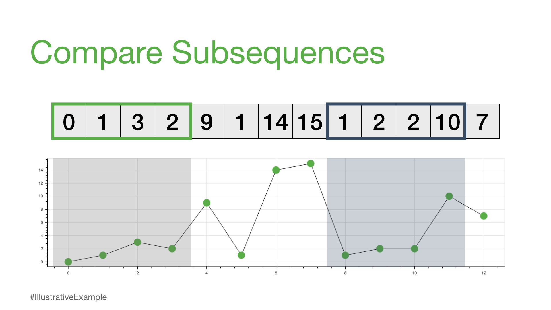
One way to compare any two subsequences is to calculate what is called the Euclidean distance.
Euclidean Distance /yo͞oˈklidēən/ /ˈdistəns/ noun#
the straight-line distance between two points#
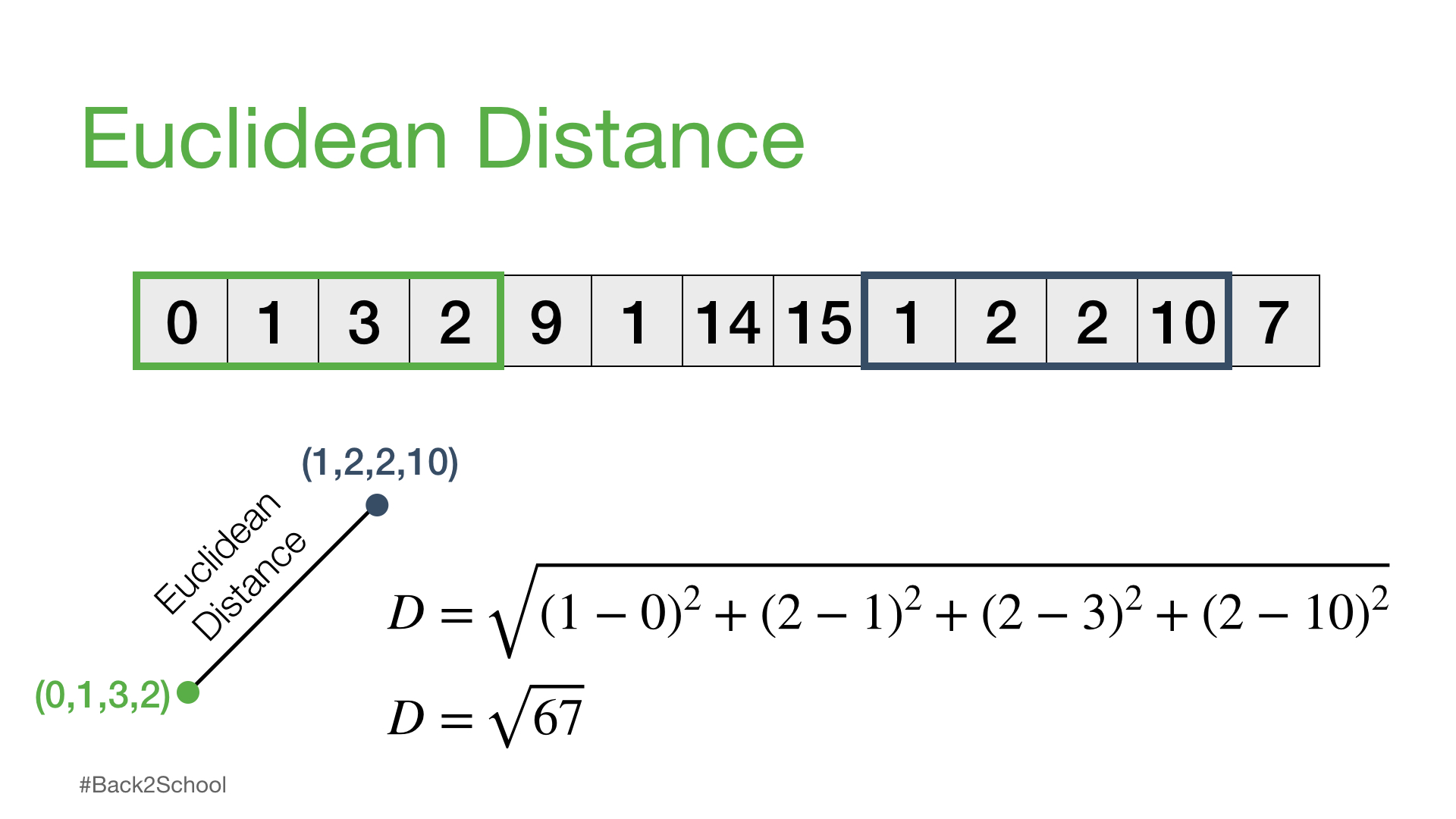
import math

D = 0
for k in range(m):
    D += (time_series[i+k] - time_series[j+k])**2
print(f"The square root of {D} = {math.sqrt(D)}")
The square root of 67 = 8.18535277187245
Distance Profile - Pairwise Euclidean Distances#
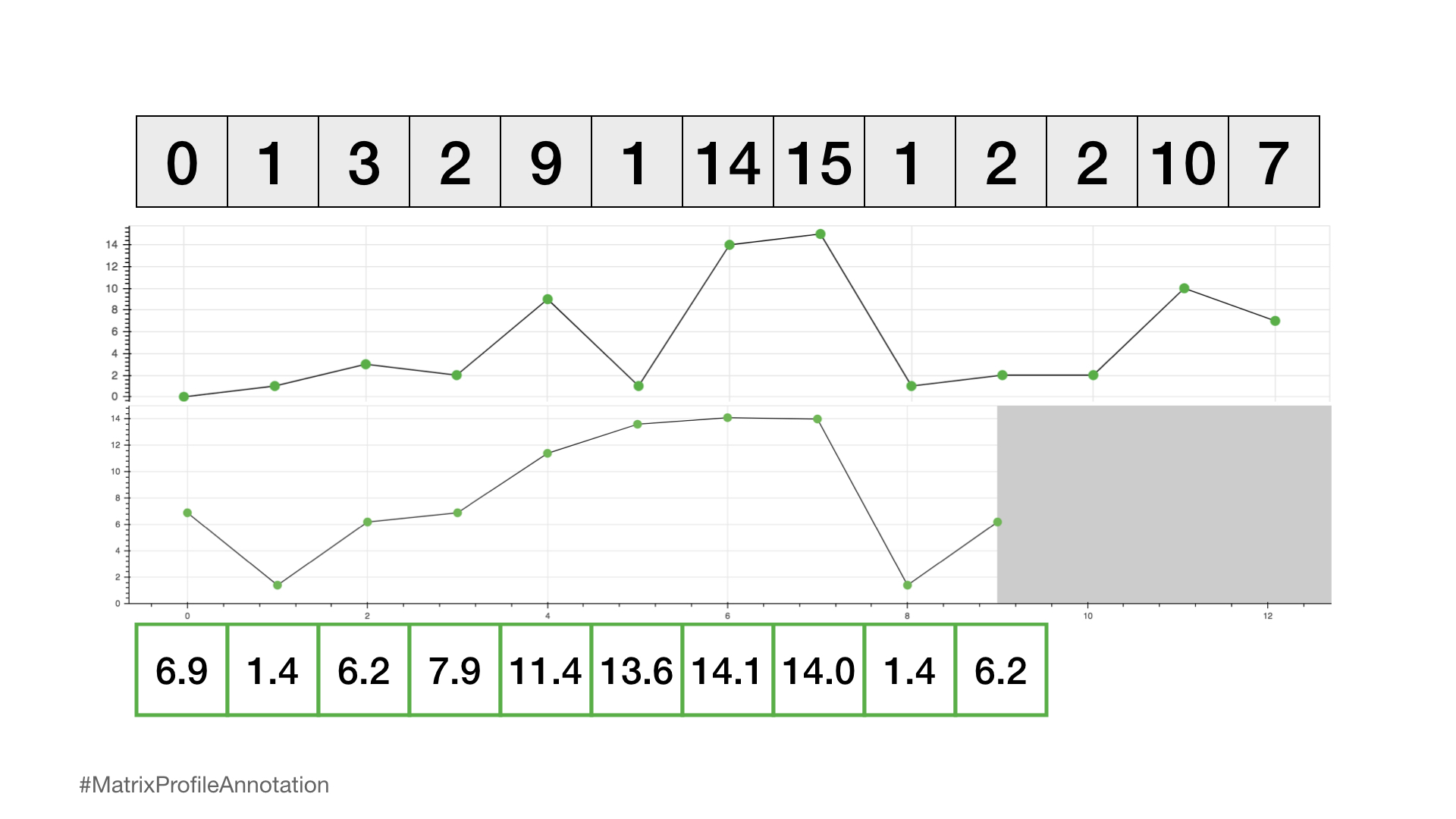
Now, we can take this a step further where we keep one subsequence the same (reference subsequence), change the second subsequence in a sliding window manner, and compute the Euclidean distance for each window. The resulting vector of pairwise Euclidean distances is also known as a distance profile.

Of course, not all of these distances are useful. Specifically, the distance for the self match (or trivial match) isn’t informative since the distance will be always be zero when you are comparing a subsequence with itself. So, we’ll ignore it and, instead, take note of the next smallest distance from the distance profile and choose that as our best match:
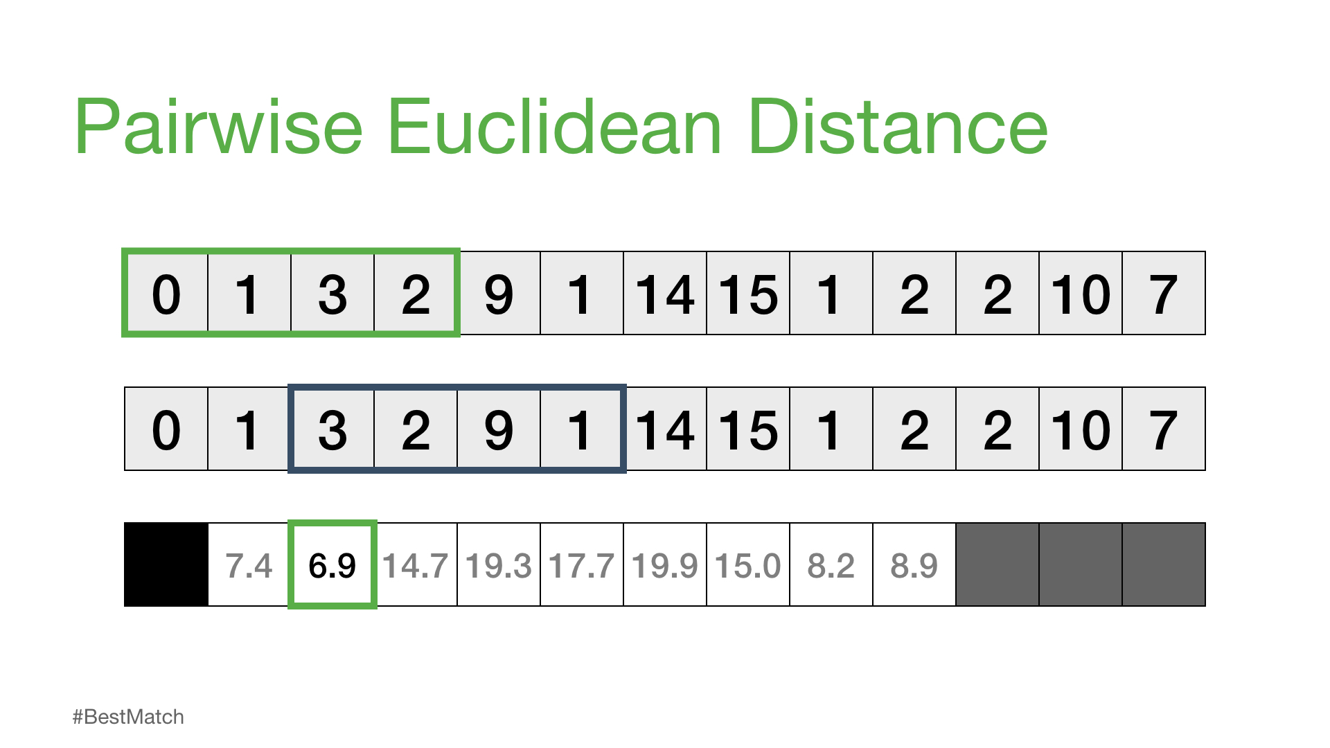
Next, we can shift our reference subsequence over one element at a time and repeat the same sliding window process to compute the distance profile for each new reference subsequence.
Distance Matrix#
If we take all of the distance profiles that were computed for each reference subsequence and stack them one on top of each other then we get something called a distance matrix
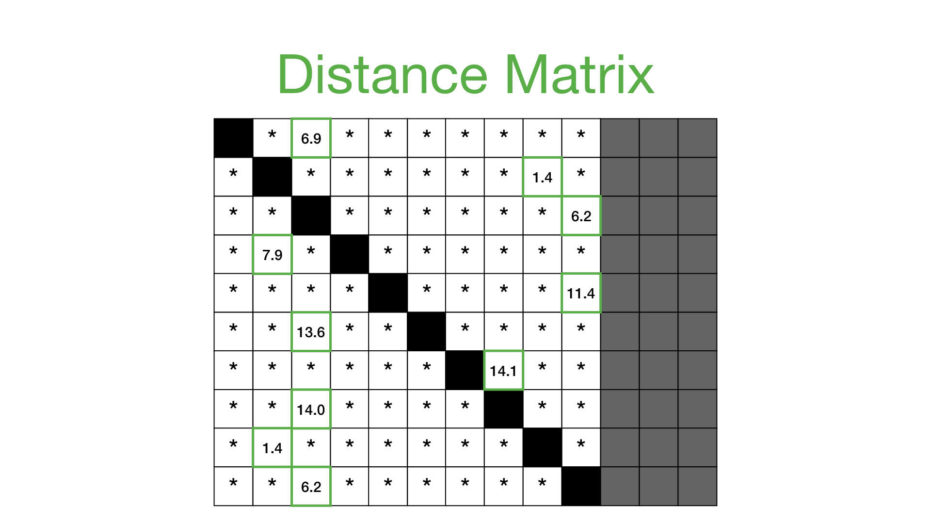
Now, we can simplify this distance matrix by only looking at the nearest neighbor for each subsequence and this takes us to our next concept:
Matrix Profile /ˈmātriks/ /ˈprōˌfīl/ noun#
a vector that stores the (z-normalized) Euclidean distance between any subsequence within a time series and its nearest neighbor#
Practically, what this means is that the matrix profile is only interested in storing the smallest non-trivial distances from each distance profile, which significantly reduces the spatial complexity to O(n):
We can now plot this matrix profile underneath our original time series. And, as it turns out, a reference subsequence with a small matrix profile value (i.e., it has a nearest neighbor significantly “closeby”) may indicate a possible pattern while a reference subsequence with a large matrix profile value (i.e., its nearest neighbor is significantly “faraway”) may suggest the presence of an anomaly.
So, by simply computing and inspecting the matrix profile alone, one can easily pick out the top pattern (global minimum) and rarest anomaly (global maximum). And this is only a small glimpse into what is possible once you’ve computed the matrix profile!
The Real Problem - The Brute Force Approach#
Now, it might seem pretty straightforward at this point but what we need to do is consider how to compute the full distance matrix efficiently. Let’s start with the brute force approach:
for i in range(n-m+1):
    for j in range(n-m+1):
        D = 0
        for k in range(m):
            D += (time_series[i+k] - time_series[j+k])**2
        D = math.sqrt(D)
At first glance, this may not look too bad but if we start considering both the computational complexity as well as the spatial complexity then we begin to understand the real problem. It turns out that, for longer time series (i.e., n >> 10,000) the computational complexity is O(n2m) (as evidenced by the three for loops in the code above) and the spatial complexity for storing the full distance matrix is O(n2).
To put this into perspective, imagine if you had a single sensor that collected data 20 times/min over the course of 5 years. This would result:
n = 20 * 60 * 24 * 364 * 5  # 20 times/min x 60 mins/hour x 24 hours/day x 365 days/year x 5 years
print(f"There would be n = {n} data points")
There would be n = 52416000 data points
Assuming that each calculation in the inner loop takes 0.0000001 seconds then this would take:
time = 0.0000001 * (n * n - n)/2
print(f"It would take {time} seconds to compute")
It would take 137371850.1792 seconds to compute
Which is equivalent to 1,598.7 days (or 4.4 years) and 11.1 PB of memory to compute! So, it is clearly not feasible to compute the distance matrix using our naive brute force method. Instead, we need to figure out how to reduce this computational complexity by efficiently generating a matrix profile and this is where STUMPY comes into play.
STUMPY#
In the fall of 2016, researchers from the University of California, Riverside and the University of New Mexico published a beautiful set of back-to-back papers that described an exact method called STOMP for computing the matrix profile for any time series with a computational complexity of O(n2)! They also further demonstrated this using GPUs and they called this faster approach GPU-STOMP.
With the academics, data scientists, and developers in mind, we have taken these concepts and have open sourced STUMPY, a powerful and scalable library that efficiently computes the matrix profile according to this published research. And, thanks to other open source software such as Numba and Dask, our implementation is highly parallelized (for a single server with multiple CPUs or, alternatively, multiple GPUs), highly distributed (with multiple CPUs across multiple servers). We’ve tested STUMPY on as many as 256 CPU cores (spread across 32 servers) or 16 NVIDIA GPU devices (on the same DGX-2 server) and have achieved similar performance to the published GPU-STOMP work.
Conclusion#
According to the original authors, “these are the best ideas in times series data mining in the last two decades” and “given the matrix profile, most time series data mining problems are trivial to solve in a few lines of code”.
From our experience, this is definitely true and we are excited to share STUMPY with you! Please reach out and let us know how STUMPY has enabled your time series analysis work as we’d love to hear from you!
Additional Notes#
For the sake of completeness, we’ll provide a few more comments for those of you who’d like to compare your own matrix profile implementation to STUMPY. However, due to the many details that are omitted in the original papers, we strongly encourage you to use STUMPY.
In our explanation above, we’ve only excluded the trivial match from consideration. However, this is insufficient since nearby subsequences (i.e., i ± 1) are likely highly similar and we need to expand this to a larger “exclusion zone” relative to the diagonal trivial match. Here, we can visualize what different exclusion zones look like:
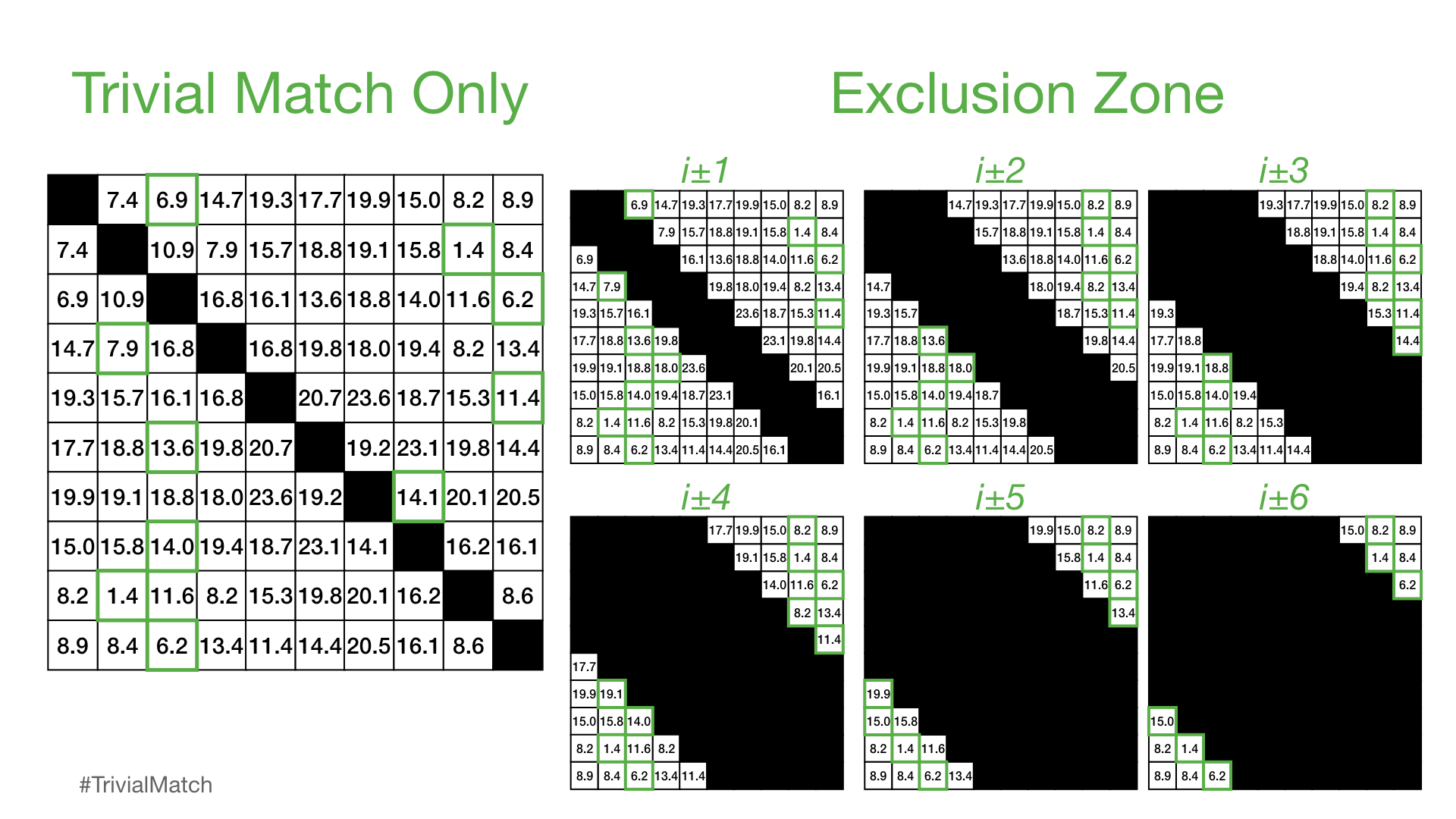
However, in practice, it has been found that an exclusion zone of i ± int(np.ceil(m / 4)) works well (where m is the subsequence window size) and the distances computed in this region are is set to np.inf before the matrix profile value is extracted for the ith subsequence. Thus, the larger the window size is, the larger the exclusion zone will be. Additionally, note that, since NumPy indexing has an inclusive start index but an exlusive stop index, the proper way to ensure a symmetrical exclusion zone is:
excl_zone = int(np.ceil(m / 4))
zone_start = i - excl_zone
zone_end = i + excl_zone + 1  # Notice that we add one since this is exclusive
distance_profile[zone_start : zone_end] = np.inf
Finally, it is very uncommon for users to need to change the default exclusion zone. However, in exceptionally rare cases, the exclusion zone can be changed globally in STUMPY through the config.STUMPY_EXCL_ZONE_DENOM parameter where all exclusion zones are computed as i ± int(np.ceil(m / config.STUMPY_EXCL_ZONE_DENOM)):
import stumpy
from stumpy import config

config.STUMPY_EXCL_ZONE_DENOM = 4  # The exclusion zone is i ± int(np.ceil(m / 4)) and is the same as the default setting
mp = stumpy.stump(T, m)

config.STUMPY_EXCL_ZONE_DENOM = 1  # The exclusion zone is i ± m
mp = stumpy.stump(T, m)

config.STUMPY_EXCL_ZONE_DENOM = np.inf  # The exclusion zone is i ± 0 and is the same as applying no exclusion zone
mp = stumpy.stump(T, m)