Shapelet Discovery

This tutorial explores the “Shapelet Discovery” case study from the research paper: The Swiss Army Knife of Time Series Data Mining: Ten Useful Things You Can Do with the Matrix Profile and Ten Lines of Code” (see Section 3.7). Also, you may want to refer to the Matrix Profile I and Time Series Shapelets: A New Primitive for Data Mining papers for more information and other related examples.

What Is A Shapelet?

Informally, time series “shapelets” are time series subsequences which are, in some sense, maximally representative of a class. For example, imagine if you had a time series that tracked the electricity consumption being used every second by the large appliances within your home for five years. Each time you run your clothes dryer, dishwasher, or air conditioner, your power meter will record the electricity being consumed and just by looking at the time series you’ll likely be able to associate an electricity consumption “signature” (i.e., shape, duration, maximum energy usage, etc) to each appliance. These patterns may be obvious or subtle and it is their uniquely “shaped” time series subsequence that allows you to differentiate between each appliance class. Thus, these so-called shapelets may be useful for classifying unlabeled time series that contain an occurrence of the shapelet. Don’t worry if this sounds bit jargon-y as everything will hopefully become clearer through our example below.

Recent research (see above) suggest that matrix profiles can be used to efficiently identify shapelets of a particular class and so, in this tutorial, we’ll build on top of our matrix profile knowledge and demonstrate how we can use STUMPY to easily discover interesting shapelets in only a few lines of additional code.

Getting Started

Let’s import the packages that we’ll need to load, analyze, and plot the data and, later, to build simple decision tree models.

%matplotlib inline

import stumpy
import pandas as pd
import numpy as np
import matplotlib.pyplot as plt
from sklearn import tree
from sklearn import metrics

plt.style.use('https://raw.githubusercontent.com/TDAmeritrade/stumpy/main/docs/stumpy.mplstyle')

Loading the GunPoint Dataset

This dataset is a motion capture time series that tracks the movement of an actors’ right hand and contains two classes:

1. Gun

2. Point

In the Gun class, the actors draw a physical gun from a hip-mounted holster, point the gun at a target for approximately one second, then return the gun to the holster, and relax their hands to their sides. In the Point class, the actors leave their gun by their sides and, instead, they point their index fingers toward the target (i.e., without a gun) for approximately one second, and then return their hands to their sides. For both classes, the centroid of the actors’ right hand was tracked to represent its motion.

Below, we’ll retrieve the raw data, split them into the gun_df and the point_df, and then, for each respective class, concatenate all of the individual samples into one long time series. Additionally, we establish a clear boundary for each sample (i.e., where a sample starts and ends) by appending a NaN value after each sample. This helps to ensure that all matrix profile computations do not return artificial subsequences that span across multiple samples:

train_df = pd.read_csv("https://zenodo.org/record/4281349/files/gun_point_train_data.csv?download=1")

gun_df = train_df[train_df['0'] == 0].iloc[:, 1:].reset_index(drop=True)
gun_df = (gun_df.assign(NaN=np.nan)
                .stack(dropna=False).to_frame().reset_index(drop=True)
                .rename({0: "Centroid Location"}, axis='columns')
         )

point_df = train_df[train_df['0'] == 1].iloc[:, 1:].reset_index(drop=True)
point_df = (point_df.assign(NaN=np.nan)
                    .stack(dropna=False).to_frame().reset_index(drop=True)
                    .rename({0: "Centroid Location"}, axis='columns')
           )

Visualizing the GunPoint Dataset

Next, let’s plot our data and visualize the differences in motion when a gun is absent and when it is physically present:

fig, axs = plt.subplots(2, sharex=True, gridspec_kw={'hspace': 0})
plt.suptitle('Point vs. Gun', fontsize='30')
plt.xlabel('Time', fontsize ='20')
fig.text(0.09, 0.5, 'Centroid Location', va='center', rotation='vertical', fontsize='20')

axs[0].plot(point_df, label="Point")
axs[0].legend()

axs[1].plot(gun_df, color="C1", label="Gun")
axs[1].legend()

plt.show()

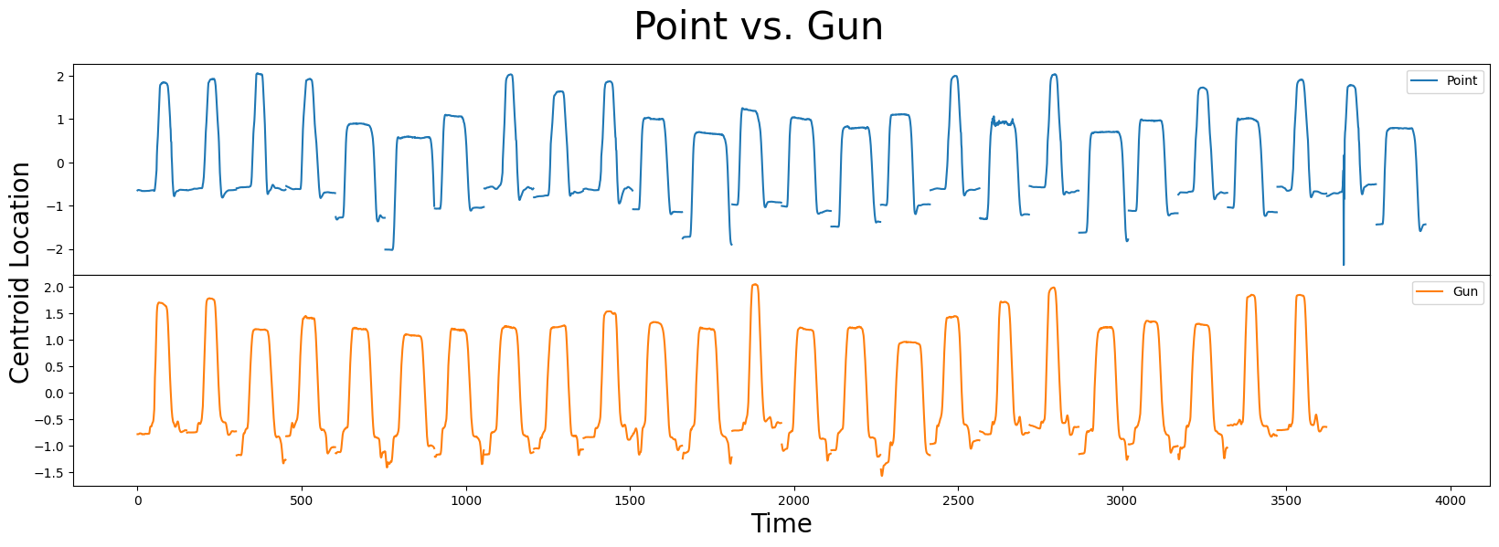
In this dataset, you’ll see that there are 26 and 24 samples for Point and Gun, respectively. Both classes contain narrow/wide samples and vertically shifted centroid locations that make it challenging to differentiate between them. Are you able to identify any subtle differences (i.e., shapelets) between Point and Gun that might help you distinguish between the two classes?

It turns out that matrix profiles may be able useful in helping us automatically identify potential shapelets!

Finding Candidate Shapelets With Matrix Profiles

Recall from our Finding Conserved Patterns Across Two Time Series Tutorial, that a matrix profile, \(P_{AA}\), calculated from a single time series, \(T_A\), is called a “self-join” and allows you to identify conserved subsequences within \(T_A\). However, a matrix profile, \(P_{AB}\), computed across two different time series, \(T_A\) and \(T_B\), is more commonly referred to as an “AB-join”. Essentially, an AB-join compares all of the subsequences in \(T_A\) with all of the subsequences in \(T_B\) in order to determine if there are any subsequences in \(T_A\) that can also be found in \(T_B\). In other words, the resulting matrix profile, \(P_{AB}\), annotates every subsequence in \(T_A\) with its best matching subsequence in \(T_B\). In contrast, if we swap the time series and compute \(P_{BA}\) (i.e., a “BA-join”), then this annotates every subsequence in \(T_B\) with its nearest neighbor subsequence in \(T_A\).

According to Section H of the Matrix Profile I paper, it is claimed that we can utilize matrix profiles to heuristically “suggest” candidate shapelets and the main intuition is that if a discriminative pattern is present in the Gun class but not in the Point class (or vice versa), then we would expect to see one or more “bumps” in their corresponding \(P_{Point,Point}\), \(P_{Point,Gun}\) (or \(P_{Gun, Gun}\), \(P_{Gun,Point}\)) matrix profiles and any significant differences in the heights may be strong indicators of good candidate shapelets.

So, first, let’s compute the matrix profiles, \(P_{Point, Point}\) (self-join) and \(P_{Point, Gun}\) (AB-join), and, for simplicity, we use a subsequence length of m = 38, which is the length of the best shapelet reported for this dataset:

m = 38
P_Point_Point = stumpy.stump(point_df["Centroid Location"], m)[:, 0].astype(float)
P_Point_Gun = stumpy.stump(point_df["Centroid Location"], m, gun_df["Centroid Location"], ignore_trivial=False)[:, 0].astype(float)

Since we have some np.nan values in the our time series, the output of the matrix profiles will contain several np.inf values. Thus, we’ll adjust this manually by converting them to np.nan:

P_Point_Point[P_Point_Point == np.inf] = np.nan
P_Point_Gun[P_Point_Gun == np.inf] = np.nan

and now we’ll plot them overlaid one on top of the other:

plt.plot(P_Point_Point, label="$P_{Point,Point}$")
plt.plot(P_Point_Gun, color="C1", label="$P_{Point,Gun}$")
plt.xlabel("Time", fontsize="20")
plt.ylabel("Matrix Profile", fontsize="20")
plt.legend()
plt.show()

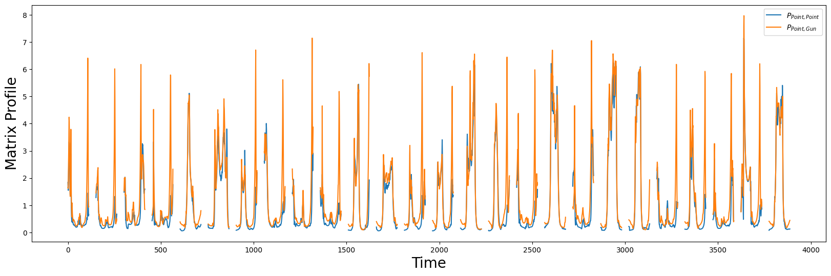
Next, we can highlight the major deviations between the two matrix profiles by plotting the difference between \(P_{Point, Point}\) and \(P_{Point, Gun}\). Intuitively, \(P_{Point, Point}\) will be smaller than \(P_{Point, Gun}\) because we would expect subsequences within the same class to be more similar than those of different classes:

P_diff = P_Point_Gun - P_Point_Point

idx = np.argpartition(np.nan_to_num(P_diff), -10)[-10:]  # get the top 10 peak locations in P_diff
plt.suptitle("", fontsize="30")
plt.xlabel("Time", fontsize="20")
plt.ylabel("$P_{diff} = P_{Point,Gun} - P_{Point, Point}$", fontsize="20")
plt.plot(idx, P_diff[idx], color="C1", marker="o", linewidth=0, markersize=10)
plt.plot(P_diff)
plt.show()

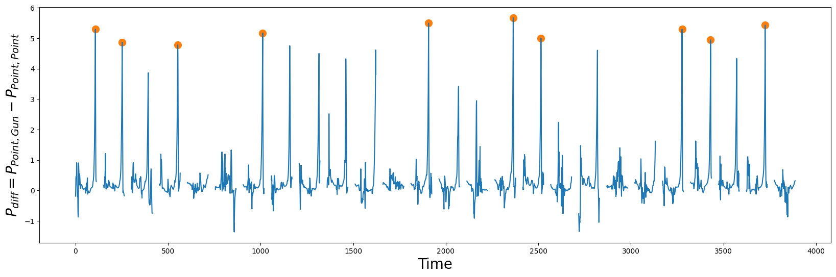
The peak values in \(P_{diff}\) (orange circles) are indicators of good shapelet candidates because they suggest patterns that are well conserved in their own class (i.e., \(P_{Point,Point}\) self-join) but are also very different from their closest match in the other class (i.e., \(P_{Point, Gun}\) AB-join). Armed with this knowledge, let’s extract the discovered shapelets and then plot them:

point_shapelets = []
for i in idx:
    shapelet = point_df.iloc[i : i + m, 0]
    point_shapelets.append(shapelet)

plt.xlabel("Time", fontsize="20")
plt.ylabel('Centroid Location', fontsize='20')
plt.plot(point_df, label="Point")
for i, shapelet in zip(idx, point_shapelets):
    plt.plot(range(i, i + m), shapelet, color="C1", linewidth=3.0)
plt.legend()
plt.show()

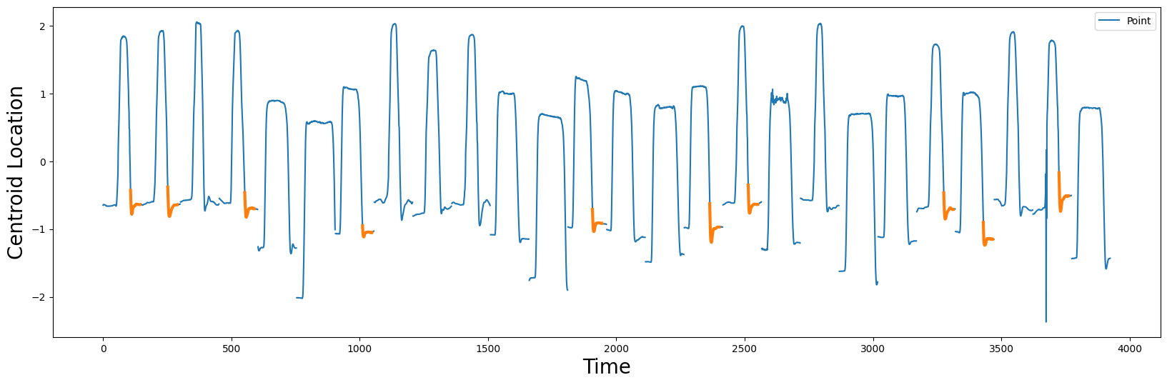
Based on these candidate shapelets (orange), it appears that the major distinguishing factor between the two classes is differentiated in how the actors’ hand returns the (imaginary) gun to the holster and then relaxes by the actors’ side. According to the original authors, the Point class “has a “dip” where the actor put her hand down by her side and it is the inertia that carries her hand a little too far and she is forced to correct for this - a phenomenon that the authors referred to as “overshooting”.

Building A Simple Classifier

Now that we’ve identified 10 candidate shapelets, let’s build 10 separate decision tree models based on these shapelets and see how well they can help us distinguish between the Point class and the Gun class. Luckily, this dataset includes a training set (above) as well as an independent test set that we can use to assess the accuracy of our models:

test_df = df = pd.read_csv("https://zenodo.org/record/4281349/files/gun_point_test_data.csv?download=1")

# Get the train and test targets
y_train = train_df.iloc[:, 0]
y_test = test_df.iloc[:, 0]

Now, for our classification task, each shapelets needs to be evaluated in terms of its predictive power. Thus, we first calculate the distance profile (pairwise Euclidean distance) between a shapelet and every subsequence within each time series or sample. Then, the smallest value is kept to understand if a close match of the shapelet in the time series has been found. The stumpy.mass function is perfectly suited for this task:

def distance_to_shapelet(data, shapelet):
    """
    Compute the minimum distance beteen each data sample and a shapelet of interest
    """
    data = np.asarray(data)
    X = np.empty(len(data))
    for i in range(len(data)):
        D = stumpy.mass(shapelet, data[i])
        X[i] = D.min()

    return X.reshape(-1, 1)

clf = tree.DecisionTreeClassifier()

for i, shapelet in enumerate(point_shapelets):
    X_train = distance_to_shapelet(train_df.iloc[:, 1:], shapelet)
    X_test = distance_to_shapelet(test_df.iloc[:, 1:], shapelet)
    clf.fit(X_train, y_train)
    y_pred = clf.predict(X_test.reshape(-1, 1))
    print(f"Accuracy for shapelet {i} = {round(metrics.accuracy_score(y_test, y_pred), 3)}")

Accuracy for shapelet 0 = 0.867
Accuracy for shapelet 1 = 0.833
Accuracy for shapelet 2 = 0.807
Accuracy for shapelet 3 = 0.833
Accuracy for shapelet 4 = 0.933
Accuracy for shapelet 5 = 0.873
Accuracy for shapelet 6 = 0.873
Accuracy for shapelet 7 = 0.833
Accuracy for shapelet 8 = 0.86
Accuracy for shapelet 9 = 0.913

As we can see, all of the shapelets provide some reasonable predictive ability that helps differentiate between the Point and Gun classes but Shapelet 4 returns the best accuracy of 93.3% and this result exactly reproduces the published findings. Great!

Bonus Section - Shapelets For The Second Class

As a little extra, we are also going to extract the shapelets from the Gun time series to see if they can add any additional predictive power to our model. The procedure is identical to the one that we’ve explained above except we are focused on shapelets derived from gun_df, so we’re not going to go into too much detail here:

m = 38
P_Gun_Gun = stumpy.stump(gun_df["Centroid Location"], m)[:, 0].astype(float)
P_Gun_Point = stumpy.stump(gun_df["Centroid Location"], m, point_df["Centroid Location"], ignore_trivial=False)[:, 0].astype(float)

P_Gun_Gun[P_Gun_Gun == np.inf] = np.nan
P_Gun_Point[P_Gun_Point == np.inf] = np.nan

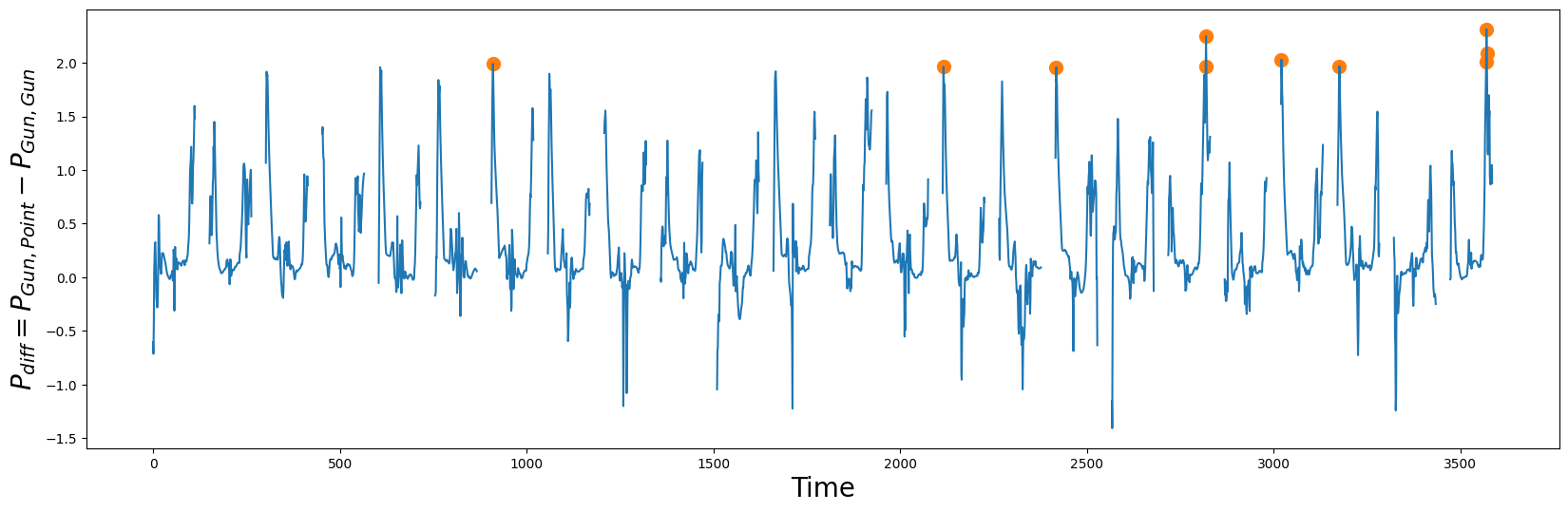
P_diff = P_Gun_Point - P_Gun_Gun

idx = np.argpartition(np.nan_to_num(P_diff), -10)[-10:]  # get the top 10 peak locations in P_diff
plt.suptitle("", fontsize="30")
plt.xlabel("Time", fontsize="20")
plt.ylabel("$P_{diff} = P_{Gun, Point} - P_{Gun, Gun}$", fontsize="20")
plt.plot(idx, P_diff[idx], color="C1", marker="o", linewidth=0, markersize=10)
plt.plot(P_diff)
plt.show()

gun_shapelets = []
for i in idx:
    shapelet = gun_df.iloc[i : i + m, 0]
    gun_shapelets.append(shapelet)

plt.xlabel("Time", fontsize="20")
plt.ylabel('Centroid Location', fontsize='20')
plt.plot(gun_df, label="Gun")
for i, shapelet in zip(idx, gun_shapelets):
    plt.plot(range(i, i + m), shapelet, color="C1", linewidth=3.0)
plt.legend()
plt.show()

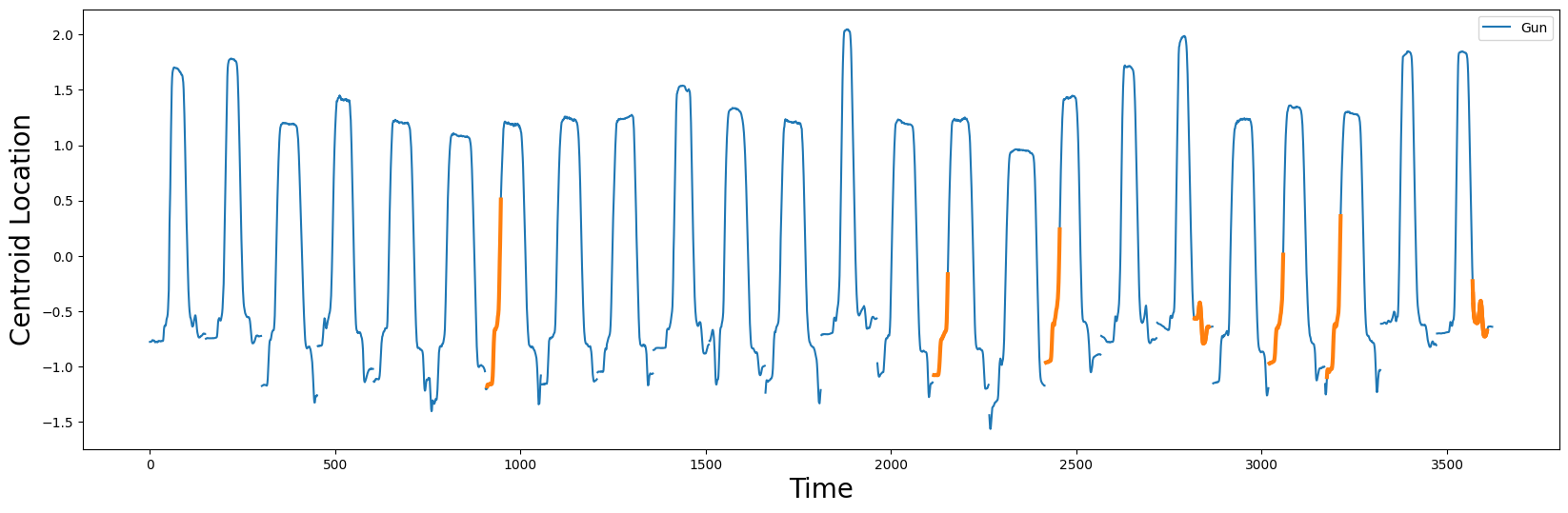
Notice that when a physical gun is present, the shapelets discovered at the beginning of the Gun drawing action aren’t as smooth as the Point samples. Similarly, re-holstering the Gun also appears to require a bit of fine adjustment.

Finally, we build our models but, this time, we combine the distance features from both the Gun shapelets as well as the Point shapelets:

clf = tree.DecisionTreeClassifier()

for i, (gun_shapelet, point_shapelet) in enumerate(zip(gun_shapelets, point_shapelets)):
    X_train_gun = distance_to_shapelet(train_df.iloc[:, 1:], gun_shapelet)
    X_train_point = distance_to_shapelet(train_df.iloc[:, 1:], point_shapelet)
    X_train = np.concatenate((X_train_gun, X_train_point), axis=1)
    X_test_gun = distance_to_shapelet(test_df.iloc[:, 1:], gun_shapelet)
    X_test_point = distance_to_shapelet(test_df.iloc[:, 1:], point_shapelet)
    X_test = np.concatenate((X_test_gun, X_test_point), axis=1)
    clf.fit(X_train, y_train)
    y_pred = clf.predict(X_test)
    print(f"Accuracy for shapelet {i} = {round(metrics.accuracy_score(y_test, y_pred), 3)}")

Accuracy for shapelet 0 = 0.913
Accuracy for shapelet 1 = 0.853
Accuracy for shapelet 2 = 0.813
Accuracy for shapelet 3 = 0.953
Accuracy for shapelet 4 = 0.933
Accuracy for shapelet 5 = 0.94
Accuracy for shapelet 6 = 0.873
Accuracy for shapelet 7 = 0.867
Accuracy for shapelet 8 = 0.867
Accuracy for shapelet 9 = 0.913

We can see that if we include both distances from Gun class shapelets and Point class shapelets, the classifier reaches 95.3% accuracy (Shapelet 3)! Apparently, adding the distances from the second class as well provides the model with additional useful information. This is a great result as it improves the result by roughly 2%. Again, it is impressive to note that all of this information can be extracted for “free” by leveraging matrix profiles.

Summary

And that’s it! You’ve just learned how to leverage matrix profiles to find shapelets and use them to build a machine learning classifier.

References

The Swiss Army Knife of Time Series Data Mining: Ten Useful Things You Can Do With The Matrix Profile And Ten Lines Of Code (see Section 3.7)

Time Series Shapelets: A New Primitive for Data Mining

STUMPY Documentation

STUMPY Matrix Profile Github Code Repository